📐 [archived] Deming versus simple linear regression
All courses that somehow covered regression models were starting almost in the same way: given bunch of $y$’s and $x$’s points, one needs to predict a value of $y$ for a certain $x$. Sounds quite easy. Without utilizing any statistical assumptions, we can just find the line, which is in a way closest to those points (best fit line).
Disclaimer: This post is outdated and was archived for back compatibility: please use with care! This post does not reflect the author’s current point of view and might deviate from the current best practices.
So the model is as follows:
\[y \approx \beta_0 + \beta_1 x\]Then typically a professor of a course leads to idea of minimizing the distances between observed variables and the fitted ones, i.e.:
\[\sum_{i=1}^n(y_i - (\beta_0 + \beta_1 x_i))\]But those distances might be both positive or negative. Thus, we need to use the absolute values, or equivalently squaring those distances, which eases the optimization problem:
\[\sum_{i=1}^n(y_i - (\beta_0 + \beta_1 x_i))^2\]Minimizing this term yields so-called linear or more commonly ordinary least squares (OLS) estimates.
So far, we did not use any of statistical assumptions. Of course due to world imperfection the relation between $y$ and $x$ is not exact and incorporates errors. These errors are modeled by the presence of randomness. Let’s define the other model, which includes a random term referred as error or disturbance term:
\[y = \beta_0 + \beta_1 x + \epsilon\]Imposing assumptions on $\epsilon$ the theoretical distribution of $y$ is known. If, furthermore, one has a sample, it is possible to utilize a powerful machinery of maximum likelihood estimation (MLE) method. It turns out that with several assumptions (homoscedastic, normal and uncorrelated errors) MLE is identical (!) to OLS (see Bradley 1973). I do not about you, but this fact shows the whole beauties of mathematics to me.
So far so good, but let’s step back for a second and check ourselves. Minimizing the distances between observed variables and the fitted ones sounds very good, but wait a second… That’s how the vertical distance defined, not the orthogonal. By definition, the shortest distance between a point and a line is actually orthogonal distance, not the vertical one, which is minimized by the OLS (see illustration below).
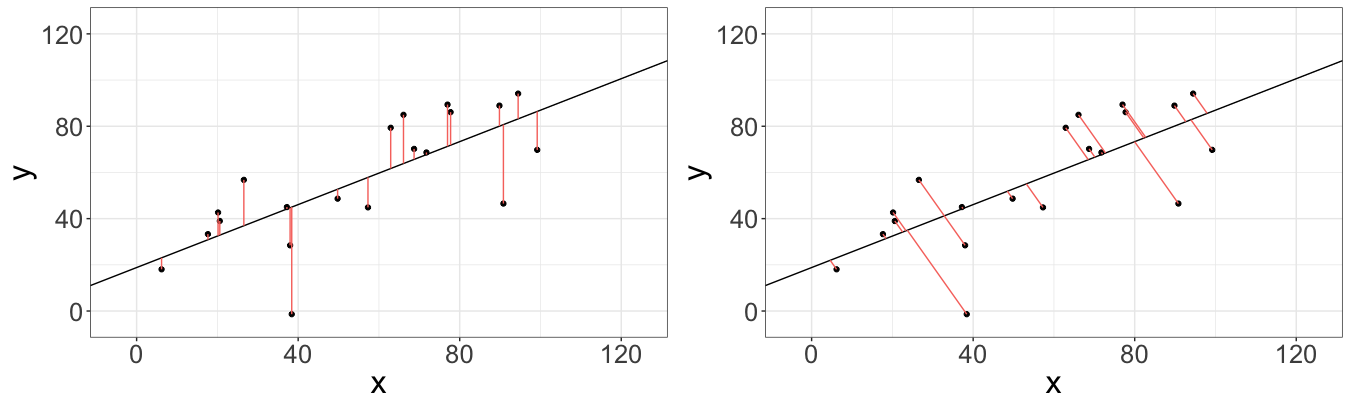
What if we minimize the orthogonal distances instead? It turns out that such model exists and is called Deming regression (even though the model was proposed by Adcock R. J. in 1878, and later being mainstreamed by Deming W.E.). The model is extremely popular in clinical chemistry nowadays.
Again, so far we did not impose any statistical assumptions. If we do so, the beauties arise again: nuts, but true – the solution of minimizing orthogonal distances is identical to MLE of errors-in-variables model with $\sigma = 1$. In this model, the data generated by the same regression model as before:
\[y^* = \beta_0 + \beta_1 x^*\]However, the observations include measurement error, i.e. we observe the following points:
\[\begin{eqnarray} y_i = y_i^* + \epsilon_i,\\ x_i = x_i^* + \eta_i, \end{eqnarray}\]For the MLE estimates that coincide with minimization solution we require:
\[\sigma = \frac{\sigma_{\epsilon}^2}{\sigma_{\eta}^2}=1\]The function deming in the package deming returns the object of class deming (a little bit too much, huh?), which contains the estimates of coefficients and other useful fields. Let’s focus on coefficients and see, whether or not Deming regression outperforms the regular OLS, if Demings’ assumptions are satisfied. For this we generate sample data according to Deming model and calibrate two regression models, Deming and simple linear one:
packages <- c("deming", "ggplot2")
# install.packages(packages)
sapply(packages, library, character.only = TRUE, logical.return = TRUE)

set.seed(20170824)

b0 <- 70
b1 <- 0.5

x_ <- runif(n = 100, min = 0, max = 100)
y_ <- b0 + b1 * x_

x <- x_ + rnorm(100, 0, 20)
y <- y_ + rnorm(100, 0, 20)

fit_ols <- lm(y ~ x)
fit_deming <- deming(y ~ x)
We need to keep estimated coefficients in a separate data frame.
(coefs <- data.frame(intercept = c(fit_ols$coefficients[1],
                                   fit_deming$coefficients[1]),
                     slope = c(fit_ols$coefficients[2],
                               fit_deming$coefficients[2]),
                     Type = factor(c("OLS", "Deming"))))
  intercept     slope   Type
1  77.76253 0.4040986    OLS
2  71.32021 0.5339840 Deming
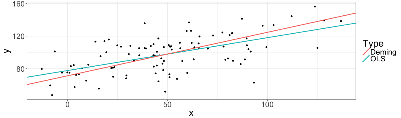
Indeed, the Demings’ coefficients are less biased than one returned by OLS. Let’s plot data with both fitted lines:
ggplot(data.frame(x = x, y = y)) +
    geom_point(aes(x = x, y = y)) +
    geom_abline(data = coefs,
                mapping = aes(intercept = intercept,
                              slope = slope,
                              colour = Type),
                size = 1) +
    theme(text = element_text(size = 24))
However, until now we worked only with one sample. The following code generates $100$ samples, fits $200$ regressions and returns data frames, which contain the relative errors of estimates for both regressions (basically we copy-pasted the old code in for loop).
set.seed(20170824)

b0 <- 70
b1 <- 0.5

n <- 100

intercept_errors <- data.frame(OLS = numeric(n),
                           Deming = numeric(n))
slope_errors <- data.frame(OLS = numeric(n),
                           Deming = numeric(n))

for(i in seq_len(n)) {
    x_ <- runif(n = 100, min = 0, max = 100)
    y_ <- b0 + b1 * x_

    x <- x_ + rnorm(100, 0, 20)
    y <- y_ + rnorm(100, 0, 20)

    fit_ols <- lm(y ~ x)
    fit_deming <- deming(y ~ x)

    intercept_errors[i, "OLS"] <- (b0 - fit_ols$coefficients[1]) / b0
    intercept_errors[i, "Deming"] <- (b0 - fit_deming$coefficients[1]) / b0

    slope_errors[i, "OLS"] <- (b1 - fit_ols$coefficients[2]) / b1
    slope_errors[i, "Deming"] <- (b1 - fit_deming$coefficients[2]) / b1

}

colMeans(slope_errors)
        OLS      Deming
0.338362764 0.000553944
colMeans(intercept_errors)
          OLS        Deming
-0.1205587030 -0.0008098469
Errors of Deming regression estimates are substantively smaller than those by OLS. As summary, it is necessary to understand, that Deming regression is useful, when both the outcome and independent variables are subjects to measurement errors. Then, it makes sense to use such a model.