🏠 [archived] Dortmund real estate market analysis: GLM and GAM

This post is dedicated to model prices of real estate by an area and a number of rooms using generalized linear model (GLM) and generalized additive model (GAM). Previous post shows how data was obtained, while in the other post the linear model is fitted to the data.

Disclaimer: This post is outdated and was archived for back compatibility: please use with care! This post does not reflect the author’s current point of view and might deviate from the current best practices.

Prices of real estates are not normally distributed, i.e. the distribution is skewed and positive. This fact was the motivation to transform the outcome variable. The alternative approach is to calibrate so-called generalized linear models, which allows the dependent variable to have other than normal distributions from exponential family.

Let’s compare the the histogram of price with theoretical densities of several distribution of exponential family. First off, we need to load several packages, set global parameters for ggplo2, clean the global environment, and load the data:

packages <- c("ggplot2", "mgcv", "magrittr", "vtreat", "MASS", "statmod",
              "dplyr", "tidyr")
sapply(packages, library, character.only = TRUE, logical.return = TRUE)

theme_set(theme_bw())
theme_update(text = element_text(size = 24))

rm(list = ls())

setwd("/Users/irudnyts/Documents/data/")
property <- read.csv("dortmund.csv")

The outcome variable price is continuous, therefore, it is natural to model it with continuous distribution. In GLM framework, two distribution are typically used, namely, gamma and inverse Gaussian (IG). Before plotting theoretical densities we need to estimate their parameters with MASS::fitdistr. For gamma distribution MASS::fitdistr does not require the initial parameters for optimization. For IG the initial parameters are found by using method of moments.

property_dens <- data.frame(price = property$price)
m <- mean(property_dens$price)
v <- var(property_dens$price)

gamma_param <- fitdistr(x = property_dens$price, densfun = "gamma")[[1]]
invgauss_param <- fitdistr(x = property_dens$price, densfun = dinvgauss,
                           start = list(mean = m, shape = m ^ 3 / v))[[1]]

property_dens <- property_dens %>%
    mutate(
        gamma = dgamma(x = price, gamma_param[1], gamma_param[2]),
        invgauss = dinvgauss(x = price, invgauss_param[1], invgauss_param[2])
    ) %>%
    gather(
        key = distr, value = dens, gamma, invgauss
    )

ggplot(property, aes(x = price)) +
    geom_density() +
    geom_line(data = property_dens,
              aes(x = price, y = dens, colour = distr))

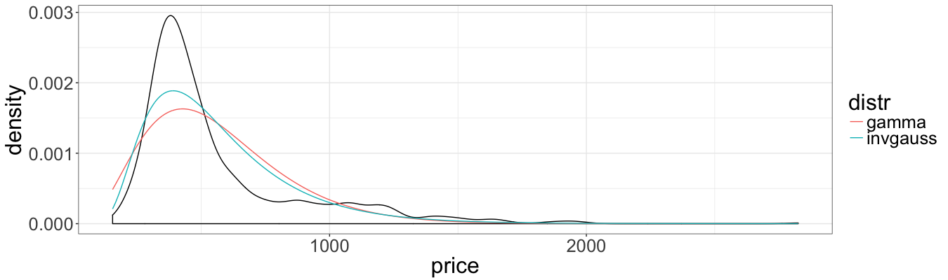
The plot indicates better fit of IG distribution. However, one should notice that the fit ignores the effect of explanatory variables, and does not fully reflect the goodness-of-fit of final regression models.

To measure goodness-of-fit we use RMSE (root mean square error), the function of which for GLM is defined below.

rmse_glm <- function(model, data = property, outcome = "price") {
    (data[, outcome] - predict(model, data, type = "response")) ^ 2 %>%
        mean() %>% sqrt()
}

Furthermore, as in the linear regression post, we want to include several interactions terms and find the optimal combination. We define different formulas and fit gamma and IG GLM. We use log link function instead of the canonical ones (inverse and inverse squared for gamma and IG, respectively). First, only log link and identity link functions yield allow the simple interpretation. Second, for gamma distribution the estimates did not converge.

formulas <- list(price ~ area,
                 price ~ area + rooms,
                 price ~ area + rooms + I(area * rooms),
                 price ~ area + rooms + I(area * rooms) + I(area / rooms),
                 price ~ area + rooms + I(area * rooms) + I(rooms / area),
                 price ~ area + rooms + I(area * rooms) + I(area / rooms) +
                     I(rooms / area)
                 )

gamma_models <- lapply(formulas, glm, data = property,
                       family = Gamma(link = "log"))
ig_models <- lapply(formulas, glm, data = property,
                    family = inverse.gaussian(link = "log"))

We extract AIC and RMSE from gamma GLM:

sapply(gamma_models, function(x) x$aic)
# [1] 10959.60 10936.19 10897.20 10899.06 10895.32 10897.07
sapply(gamma_models, function(x) rmse_glm(x))
# [1] 368.8411 373.2765 181.2491 180.7917 171.4788 171.0334

In terms of AIC, the model with area, rooms and interaction terms area * rooms and rooms / area is the optimal one. Even though the minimal RMSE is returned by the model including all interaction terms, we chose the optimal one by AIC.

The same procedure is done for IF GLM:

sapply(ig_models, function(x) x$aic)
# [1] 10879.90 10850.35 10850.98 10852.87 10851.65 10853.59
sapply(ig_models, function(x) rmse_glm(x))
# [1] 418.4236 455.3432 324.5220 327.3428 357.5091 358.4135

For IG GLM, both AIC and RMSE suggest to use model with price, rooms and interaction rooms * area. Note that IG returns much larger RMSE, and from this perspective gamma GLM is preferred. However, before stepping further let’s see models perform with out-of-sample prediction. We again use cross-validation techniques.

cv_rmse <- function(folds, fit_function, fit_formula, fit_data, fit_family) {
    pred <- rep(NA, nrow(fit_data))
    for(fold in folds) {
        fit_model <- fit_function(data = fit_data[fold$train, ],
                           formula = fit_formula,
                           family = fit_family)
        pred[fold$app] <- predict(fit_model,
                                  fit_data[fold$app, ],
                                  type = "response")
    }
    (fit_data[, all.vars(fit_formula)[1]] - pred) ^ 2 %>% mean() %>% sqrt()
}

set.seed(3)
folds <- kWayCrossValidation(nRows = nrow(property), nSplits = 3)

cv_rmse(folds = folds,
        fit_function = glm,
        fit_formula = formulas[[5]],
        fit_data = property,
        fit_family = Gamma(link = "log"))
# [1] 193.8105
cv_rmse(folds = folds,
        fit_function = glm,
        fit_formula = formulas[[3]],
        fit_data = property,
        fit_family = inverse.gaussian(link = "log"))
# [1] 311.6875

Gamma GLM is still better that IG. At the same time, IG shows lower out-of-sample than in-sample RMSE. It indicates that IG GLM is not overfitted.

So far, we fitted two GLM models, none of which is better than a simple linear regression in terns of RMSE.

The further extension of GLM is generalized additive models (GAM) that allow the linear predictor be dependent on (smooth) functions of predictors.

gam_gamma_model <- gam(formula = price ~ s(area) + s(rooms),
                       family = Gamma(link = "log"), data = property)
rmse_glm(gam_gamma_model)
# [1] 132.3109

gam_ig_model <- gam(formula = price ~ s(area) + s(rooms),
                    family = inverse.gaussian(link = "log"), data = property)
rmse_glm(gam_ig_model)
# [1] 134.9973

Again, the model with underlying gamma distribution is slightly better than with IG. What cross-validation says?

cv_rmse(folds = folds,
        fit_function = gam,
        fit_formula = price ~ s(area) + s(rooms),
        fit_data = property,
        fit_family = Gamma(link = "log"))
# [1] 142.1805

cv_rmse(folds = folds,
        fit_function = gam,
        fit_formula = price ~ s(area) + s(rooms),
        fit_data = property,
        fit_family = inverse.gaussian(link = "log"))
# [1] 138.4663

The model with Gamma distribution returns higher out-of-sample RMSE than IG. Furthermore, for Gamma out-of-sample RMSE is considerably larger than in-sample, which a signal of overfitting risk. IG model in- and out-of-sample RMSE are comparable. This fact and my personal gut feeling are in favor of IG GAM. But more importantly, GAM IG shows substantially lower RMSE than all other previous models.

As summary, GLM are not always better than simple linear regression, even if the distribution of outcome variable is non-normal. In our particular case GAM significantly improves RMSE.