🍺 [archived] Dortmund real estate market analysis: linear regression models
In this post we use various linear regression models to describe the real estate market in Dortmund. The process of tidying and obtaining data can be found in previous post, while the data can be downloaded from gist.
Disclaimer: This post is outdated and was archived for back compatibility: please use with care! This post does not reflect the author’s current point of view and might deviate from the current best practices.
The data contains prices, areas, number of rooms, addresses and city parts of 888 ads. In this post we use only covariates area and rooms to predict the value of price. Of course to build a comprehensive model, one should also include factorized variable part. Due to the vast number of factors (74), for the time being we omit this variable.
Before deep diving into details, let’s calibrate a dumb model, just to have a first glance.
packages <- c("ggplot2", "tibble", "MASS", "mgcv", "magrittr", "dplyr",
              "gridExtra", "vtreat")
sapply(packages, library, character.only = TRUE, logical.return = TRUE)
# options(scipen=999)
rm(list = ls())

setwd("/Users/irudnyts/Documents/data/")
property <- read.csv("dortmund.csv")

model1 <- lm(formula = price ~ area + rooms, data = property)
summary(model1)
Call:
lm(formula = price ~ area + rooms, data = property)

Residuals:
    Min      1Q  Median      3Q     Max
-739.98  -94.91  -15.26   74.98  807.05

Coefficients:
            Estimate Std. Error t value Pr(>|t|)
(Intercept) -47.4067    17.0399  -2.782  0.00552 **
area         10.7375     0.2304  46.608  < 2e-16 ***
rooms       -67.3781     8.0927  -8.326 3.16e-16 ***
---
Signif. codes:  0 ‘***’ 0.001 ‘**’ 0.01 ‘*’ 0.05 ‘.’ 0.1 ‘ ’ 1

Residual standard error: 150.5 on 885 degrees of freedom
Multiple R-squared:  0.7855,	Adjusted R-squared:  0.785
F-statistic:  1620 on 2 and 885 DF,  p-value: < 2.2e-16
All coefficients are significant. The intercept tells not much in this case: what’s the price of the apartment with no rooms and 0-area? The positive value of area coefficient is the price of additional square meter keeping all other variables (actually only the number of rooms) constant. It’s interesting to see the negative sign of rooms coefficient. The interpretation is as follows: given, for instance, an apartment of 50 square meters, one-room apartment would cost to rent 67 euros more expensive than two-rooms apartment. Surprisingly, it goes along with intuition: apartments with larger rooms have higher rent, and we will exploit this fact later on. This model explains around 78% of the price variance. Let’s see if we can improve our predictions using other linear regression models that are the simplest models can be used. We try to extract from them everything we can.
Model selection
What variables should be included in the model? The standard procedure in R step() is an implementation of stepwise regression. This technique is heavily criticized in recent years. For instance, it is well-known, the more predictors are included in the model, the higher $R^2$. Furthermore, it make no sense to apply stepwise regression if one has only two regressor, like in our case. We focus on ANOVA and AIC tests, but first we explore the relation between covariates:
cor(property$area, property$rooms)
# 0.6877519
ggplot(data = property) +
    geom_point(aes(rooms, area)) +
    geom_smooth(aes(rooms, area), method = "loess", se = FALSE, colour = "red") +
    theme_bw() +
    theme(text = element_text(size = 24))
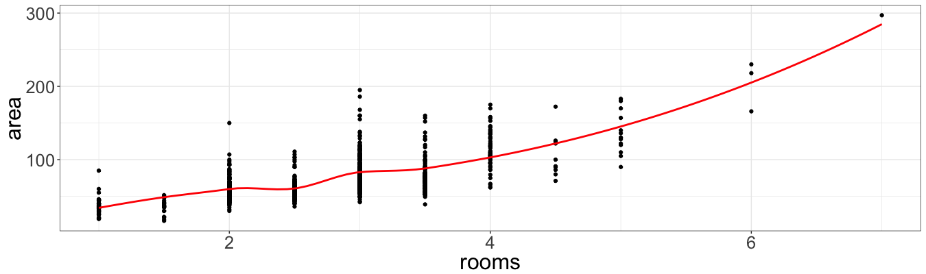
Variables area and rooms are positively correlated (which is not a big surprise), but definitely have non-linear relation. Now we must investigate if price can be predicted better by only one of these variables. Also it is necessary to check if the interaction (area * rooms) term is needed. Remember it was mentioned in the beginning, that it is reasonable to assume that the area per room might be relevant? Thus, we include this variable (area / rooms) as well. Then, why not include the opposite ratio (rooms / area)? We calibrate ten models with different sets of regressors and compare RMSE (root mean square error), $R^2$, AIC, and run ANOVA test.
models <- list(
    lm(price ~ area, property),
    lm(price ~ rooms, property),
    lm(price ~ area + rooms, property),
    lm(price ~ area + rooms + I(area * rooms), property),
    lm(price ~ area + rooms + I(area / rooms), property),
    lm(price ~ area + rooms + I(rooms / area), property),
    lm(price ~ area + rooms + I(area * rooms) + I(area / rooms), property),
    lm(price ~ area + rooms + I(area * rooms) + I(rooms / area), property),
    lm(price ~ area + rooms + I(area / rooms) + I(rooms / area), property),
    lm(price ~ area + rooms + I(rooms / area) + I(area * rooms) +
           I(area / rooms), property)
)

rmse <- function(model, data = property, outcome = "price") {
    (data[, outcome] - predict(model, data)) ^ 2 %>% mean() %>% sqrt()
}

sapply(models, rmse) %>% round(digits = 2)
# [1] 156.04 279.30 150.27 150.15 149.73 147.62 149.72 147.62 147.62 147.62
sapply(models, function(x) summary(x)$r.squared) %>% round(digits = 4) * 100
# [1] 76.87 25.90 78.55 78.58 78.70 79.30 78.71 79.30 79.30 79.30
sapply(models, AIC) %>% round(digits = 2)
# [1] 11495.07 12528.96 11430.11 11430.74 11425.71 11400.50 11427.57 11402.48
# [9] 11402.49 11404.48

anova(models[[1]], models[[3]], models[[6]], models[[8]], models[[10]])
Analysis of Variance Table

Model 1: price ~ area
Model 2: price ~ area + rooms
Model 3: price ~ area + rooms + I(rooms/area)
Model 4: price ~ area + rooms + I(area * rooms) + I(rooms/area)
Model 5: price ~ area + rooms + I(rooms/area) + I(area * rooms) + I(area/rooms)
  Res.Df      RSS Df Sum of Sq       F    Pr(>F)
1    886 21622409
2    885 20051811  1   1570598 71.5896 < 2.2e-16 ***
3    884 19350505  1    701306 31.9663 2.118e-08 ***
4    883 19350205  1       300  0.0137    0.9069
5    882 19350113  1        92  0.0042    0.9483
---
Signif. codes:  0 ‘***’ 0.001 ‘**’ 0.01 ‘*’ 0.05 ‘.’ 0.1 ‘ ’ 1
According to all criteria the model that includes only area significantly outperforms the model with only rooms. Adding the variable rooms to the model with only area tangibly improves the model. Then, surely, we could add different covariates and pair-wisely compare models, but we focus on AIC instead, which penalize those models with too many covariates. The model that includes area, rooms, and the interaction term rooms / area shows the smallest AIC, competitive $R^2$, and among the smallest RMSE. Furthermore, ANOVA test shows that adding area * rooms and area / rooms does not improve the model significantly. As long as we want to avoid overfitting, we use the model selected by AIC, i.e. with both variables (area and rooms) and the interaction term rooms / area as reference model.
Residuals and outliers diagnostics
Our data might have outliers, which bias the coefficients. Those outliers should be found, inspected, and if indeed these guys are outliers, then, thrown away. There is no out-of-the-box method how to detect outliers. One can use dozens of different measures in R built-in function influence.measures. Of course, to use them all would be an overkill, that’s why we don’t use the strict procedure. We start from plotting residuals:
ref_model <- lm(price ~ area + rooms + I(rooms / area),
                property)

ggplot(data = data.frame(n = 1:888, r = ref_model$residuals)) +
    geom_point(aes(n, r)) +
    theme_bw() +
    theme(text = element_text(size = 24))
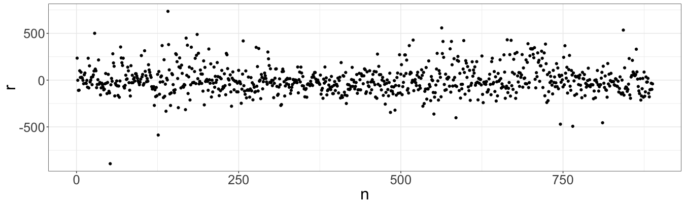
Everything looks quite smooth except two points with largest residuals, which are selected by the following code:
sort(abs(ref_model$residuals), decreasing = TRUE)[1:5]
#       52      141      126      563      843
# 893.6243 735.4020 587.2990 558.2192 534.7874
It is also possible to compare these points with points of largest hatvalues and cooks.distance. The former measures the leverage, and the later measures overall change in the coefficients when the point is not used for estimation:
sort(hatvalues(ref_model), decreasing = TRUE)[1:5]
#        590         52         62        761        747
# 0.10401959 0.09626561 0.06630276 0.06340936 0.05365715
sort(cooks.distance(ref_model), decreasing = TRUE)[1:5]
#         52        141        126        746        811
# 1.07497787 0.25812160 0.13949108 0.04843232 0.04469382
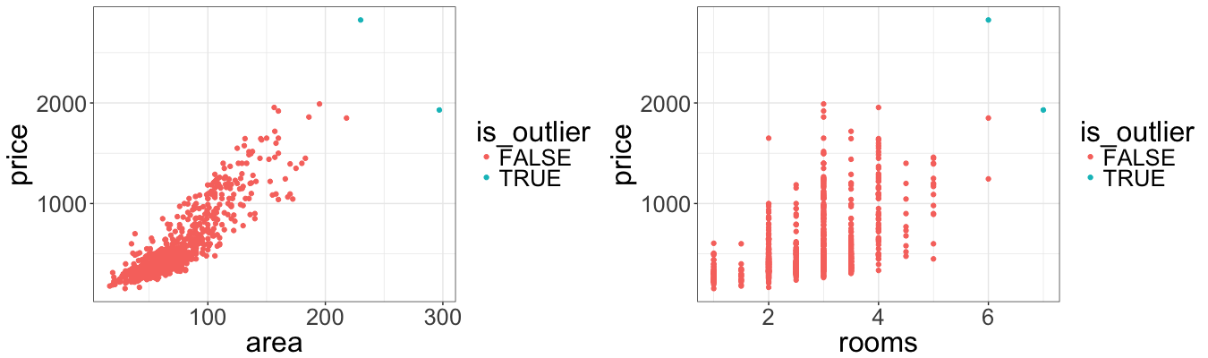
Two points (52 and 141) appear to be with largest residuals and in top five points with largest Cook’s distances. Also observation #52 has second largest hat-value. Further investigation shows that these two observations have largest area and rooms.
property[c(52, 141), 1:3]
#     price area rooms
# 52   1930  297     7
# 141  2825  230     6
property$is_outlier <- FALSE; property$is_outlier[c(52, 141)] <- TRUE
grid.arrange(
    ggplot(data = property) +
        geom_point(aes(area, price, colour = is_outlier)) +
        theme_bw() +
        theme(text = element_text(size = 24)),
    ggplot(data = property) +
        geom_point(aes(rooms, price, colour = is_outlier)) +
        theme_bw() +
        theme(text = element_text(size = 24)),
    ncol = 2
)
property[order(property$area, decreasing = TRUE), 1:3] %>% head()
#     price area rooms
# 52   1930  297     7
# 141  2825  230     6
# 666  1850  218     6
# 62   1990  195     3
# 747  1860  186     3
# 409  1450  183     5
We fit the model without such outliers. Unfortunately, AIC cannot be used for choosing the best model, since models are calibrated on different sets of data. Fitting data without outliers slightly decreases $R^2$ and increases RMSE. RMSE is also based on data without outliers, and, thus, also biased measurement. Therefore, in further analysis we keep outliers.
unb_model <- lm(price ~ area + rooms + I(rooms / area),
                property[!property$is_outlier, ])
coef(unb_model); coef(ref_model)
# (Intercept)          area         rooms I(rooms/area)
#  -300.01637      13.88343    -159.22218    6929.05469
# (Intercept)          area         rooms I(rooms/area)
#  -263.14824      13.38995    -147.71802    6109.04617
sapply(list(unb_model, ref_model),
       function(x) summary(x)$r.squared)
# [1] 0.7919386 0.7929940
sapply(list(unb_model, ref_model), rmse, data = property[!property$is_outlier, ])
# [1] 142.4912 142.5783
Transformation of response variable
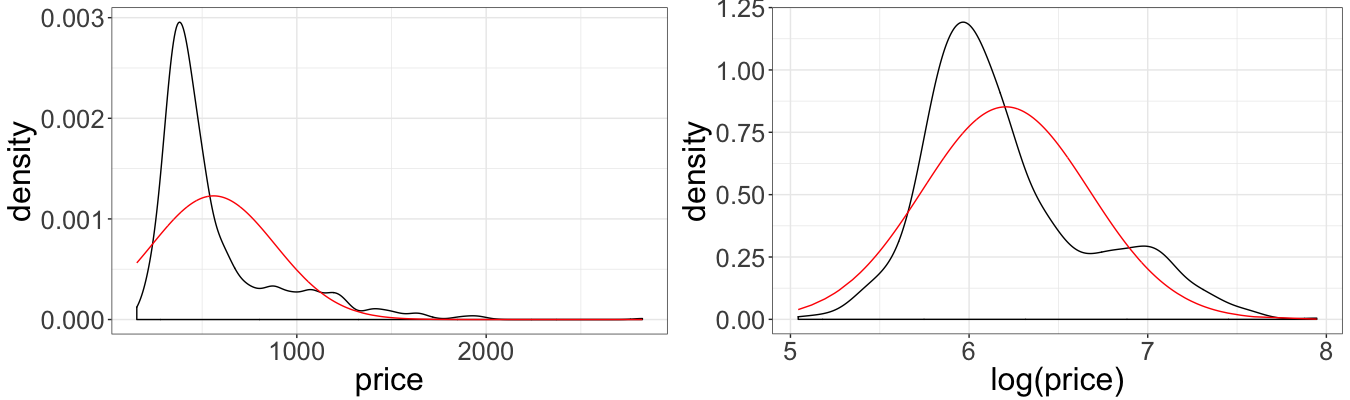
The multiple linear regression model assumes the normality of the error terms, therefore, assuming normality of the dependent variable. Obviously prices are not normal, since they are only positive values and the distribution is skewed. In this case, typically log transformation is applied to the dependent variable.
property$norm <- dnorm(property$price,
                       mean = mean(property$price),
                       sd = sd(property$price))
property$norm_log <- dnorm(log(property$price),
                           mean = mean(log(property$price)),
                           sd = sd(log(property$price)))

grid.arrange(
    ggplot(data = property) + geom_density(aes(price)) +
        geom_line(aes(price, norm), col = "red") + theme_bw() +
        theme(text = element_text(size = 24)),
    ggplot(data = property) + geom_density(aes(log(price))) +
        geom_line(aes(log(price), norm_log), col = "red") + theme_bw() +
        theme(text = element_text(size = 24)),
    ncol = 2
)
property$norm <- NULL
property$norm_log <- NULL
We agin quickly perform model selection. This time we chose the model with both variables and the multiplicative interaction term (area * rooms), as one with smallest AIC. The interaction term became significant due to the nature of logarithm transform.
log_models <- list(
    lm(log(price) ~ area, property),
    lm(log(price) ~ rooms, property),
    lm(log(price) ~ area + rooms, property),
    lm(log(price) ~ area + rooms + I(area * rooms), property),
    lm(log(price) ~ area + rooms + I(area / rooms), property),
    lm(log(price) ~ area + rooms + I(rooms / area), property),
    lm(log(price) ~ area + rooms + I(area * rooms) + I(area / rooms), property),
    lm(log(price) ~ area + rooms + I(area * rooms) + I(rooms / area), property),
    lm(log(price) ~ area + rooms + I(area / rooms) + I(rooms / area), property),
    lm(log(price) ~ area + rooms + I(rooms / area) + I(area * rooms) +
           I(area / rooms), property)
)

log_rmse <- function(log_model, data = property, outcome = "price") {
    (data[, outcome] - exp(predict(log_model, data))) ^ 2 %>% mean() %>% sqrt()
}

sapply(log_models, log_rmse) %>% round(digits = 2)
# [1] 322.33 280.02 324.38 171.77 284.05 282.96 171.35 165.09 269.22 164.94
sapply(log_models, function(x) summary(x)$r.squared) %>% round(digits = 4) * 100
# [1] 75.60 29.78 76.11 77.74 76.37 76.41 77.75 77.84 76.50 77.84
sapply(log_models, AIC) %>% round(digits = 2)
# [1]  -74.97  863.54  -92.04 -152.66  -99.50 -101.16 -151.01 -154.48 -102.42
# [10] -152.54

anova(log_models[[1]], log_models[[3]], log_models[[4]], log_models[[7]],
      log_models[[8]], log_models[[10]])
Analysis of Variance Table

Model 1: log(price) ~ area
Model 2: log(price) ~ area + rooms
Model 3: log(price) ~ area + rooms + I(area * rooms)
Model 4: log(price) ~ area + rooms + I(area * rooms) + I(area/rooms)
Model 5: log(price) ~ area + rooms + I(area * rooms) + I(rooms/area)
Model 6: log(price) ~ area + rooms + I(rooms/area) + I(area * rooms) +
    I(area/rooms)
  Res.Df    RSS Df Sum of Sq       F    Pr(>F)
1    886 47.461
2    885 46.453  1    1.0083 20.6337 6.334e-06 ***
3    884 43.290  1    3.1633 64.7319 2.759e-15 ***
4    883 43.273  1    0.0168  0.3438    0.5578
5    883 43.104  0    0.1691
6    882 43.101  1    0.0024  0.0501    0.8230
---
Signif. codes:  0 ‘***’ 0.001 ‘**’ 0.01 ‘*’ 0.05 ‘.’ 0.1 ‘ ’ 1
Let’s calibrate our reference log-transformed models and compare RMSE with the initial reference model. Note, due to the nature of the logarithm, the log-transformed model minimize Root Mean Square Relative Error (RMSRE) instead RMSE, so it makes sense to compare RMSRE as well.
log_ref_model <- lm(log(price) ~ area + rooms + I(area * rooms), property)

c(rmse(ref_model), log_rmse(log_ref_model))
# [1] 147.6181 171.7737

c(((predict(ref_model) - property$price) / property$price) ^ 2 %>%
      mean() %>% sqrt(),
  ((exp(predict(log_ref_model)) - property$price) / property$price) ^ 2 %>%
      mean() %>% sqrt())
# [1] 0.2410944 0.2222028
The log-transformed model returns higher RMSE when compared to the initial reference model, and a bit better RMSRE. In general, log-transformed model is preferred one, since it never returns negative values, even though it has larger RMSE.
Cross-validation
Finally, two models (reference and log-transformed) should be validated (tested on overfitting). For this we use k-fold cross validation techniques:
property$simple_pred <- NULL
property$log_pred <- NULL

set.seed(1)
folds <- kWayCrossValidation(nRows = nrow(property), nSplits = 3)

for(fold in folds) {
    # simple model
    simpl_model <- lm(data = property[fold$train, ],
                      formula = price ~ area + rooms + I(rooms / area))
    property[fold$app, "simple_pred"] <- predict(simpl_model,
                                                 property[fold$app, ])
    # log model
    log_model <- lm(data = property[fold$train, ],
                      formula = log(price) ~ area + rooms + I(area * rooms))
    property[fold$app, "log_pred"] <- exp(predict(log_model,
                                                 property[fold$app, ]))

}

c((property$price - property$simple_pred) ^ 2 %>% mean() %>% sqrt(),
  (property$price - property$log_pred) ^ 2 %>% mean() %>% sqrt())
# [1] 148.2719 198.9451

c(((property$price - property$simple_pred) / property$price) ^ 2 %>%
      mean() %>% sqrt(),
  ((property$price - property$log_pred) / property$price) ^ 2 %>%
      mean() %>% sqrt())
# [1] 0.2436167 0.2301364
It seems that the reference model is not overfitted, since the out-of-sample RMSE is very close to in-sample one (147.6181 and 148.2719, respectively). The same concerns to RMSRE (0.2410944 and 0.2436167). However, log-transformed model has slightly larger RMSE on test data (198.9451 against 171.7737), and more or less similar RMSRE (0.2301364 and 0.2222028).
Depending on which measure (RMSE or RMSRE) is used, one or another model is preferred. Of course, one can argue that for the reference model it’s easier to interpret coefficients. However, the log-transformed model returns only non-negative prices, which makes sense in the given context. In further posts, we will utilize the power of GLM, GAM, and tree-based methods.